QuantLearn
Trading Strategies
Heikin-Ashi Candlestick
Japanese candlestick technique for trend analysis
Backtest Performance Analysis
Historical testing on NVIDIA stock showing Heikin-Ashi strategy performance with trend following signals.
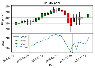
Heikin-Ashi Trading Positions
Heikin-Ashi candlestick chart with buy/sell signals marked. Note the smoother price action compared to traditional candlesticks.
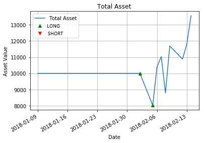
Portfolio Asset Value
Total portfolio value over time showing the impact of Heikin-Ashi trend following strategy on capital growth.
Heikin-Ashi Theory
Heikin-Ashi, meaning "Average Bar" in Japanese, is an alternative candlestick charting method designed to filter out market noise.
Unlike traditional candlesticks that use actual OHLC values, Heikin-Ashi applies mathematical transformations to create smoother price action.
The technique shows more consecutive bars of the same color, making trends and reversal points more distinguishable.
Heikin-Ashi excels in sideways and choppy markets where traditional indicators produce false signals.
The method emphasizes momentum trading by reducing the impact of gap-ups, gap-downs, and intraday volatility.
Traders use specific Heikin-Ashi candlestick patterns to determine entry and exit points with higher confidence.
Heikin-Ashi Calculations
1Heikin-Ashi Close
The HA close is the average of the four price points, providing a smoothed closing value.
2Heikin-Ashi Open (Recursive)
The HA open uses the previous period's average of HA open and close, creating momentum continuity.
3Heikin-Ashi High
The HA high is the maximum of the actual high, HA open, and HA close values.
4Heikin-Ashi Low
The HA low is the minimum of the actual low, HA open, and HA close values.
Heikin-Ashi Implementation
The algorithm transforms traditional OHLC data into Heikin-Ashi format and applies trend-following rules for signal generation.
Heikin-Ashi Transformation
def heikin_ashi(data):
    df = data.copy()
    df.reset_index(inplace=True)

    # Calculate HA close (average of OHLC)
    df['HA close'] = (df['Open'] + df['Close'] + df['High'] + df['Low']) / 4

    # Initialize HA open
    df['HA open'] = float(0)
    df['HA open'][0] = df['Open'][0]

    # Calculate HA open recursively
    for n in range(1, len(df)):
        df.at[n, 'HA open'] = (df['HA open'][n-1] + df['HA close'][n-1]) / 2

    # Calculate HA high and low
    temp = pd.concat([df['HA open'], df['HA close'], df['Low'], df['High']], axis=1)
    df['HA high'] = temp.apply(max, axis=1)
    df['HA low'] = temp.apply(min, axis=1)

    return df
Transforms regular OHLC data into Heikin-Ashi format using the mathematical formulas, creating smoother price action.
Trend Signal Generation
def signal_generation(df, method, stls):
    data = method(df)
    data['signals'] = 0
    data['cumsum'] = 0

    for n in range(1, len(data)):
        # Long signal conditions (all must be true):
        # 1. HA open > HA close (bearish candle)
        # 2. HA open == HA high (no upper shadow)
        # 3. Current body > previous body (increasing momentum)
        # 4. Previous candle was also bearish
        if (data['HA open'][n] > data['HA close'][n] and
            data['HA open'][n] == data['HA high'][n] and
            abs(data['HA open'][n] - data['HA close'][n]) >
            abs(data['HA open'][n-1] - data['HA close'][n-1]) and
            data['HA open'][n-1] > data['HA close'][n-1]):

            data.at[n, 'signals'] = 1
            data['cumsum'] = data['signals'].cumsum()

            # Stop loss limit check
            if data['cumsum'][n] > stls:
                data.at[n, 'signals'] = 0

        # Exit signal conditions:
        # 1. HA open < HA close (bullish candle)
        # 2. HA open == HA low (no lower shadow)
        # 3. Previous candle was also bullish
        elif (data['HA open'][n] < data['HA close'][n] and
              data['HA open'][n] == data['HA low'][n] and
              data['HA open'][n-1] < data['HA close'][n-1]):

            data.at[n, 'signals'] = -1
            data['cumsum'] = data['signals'].cumsum()

            # Clear all positions
            if data['cumsum'][n] > 0:
                data.at[n, 'signals'] = -1 * (data['cumsum'][n-1])
            if data['cumsum'][n] < 0:
                data.at[n, 'signals'] = 0

    return data
Generates buy/sell signals based on specific Heikin-Ashi candlestick patterns that indicate momentum continuation or reversal.
Risk Management
def portfolio(data, capital0=10000, positions=100):
    data['cumsum'] = data['signals'].cumsum()

    portfolio = pd.DataFrame()
    portfolio['holdings'] = data['cumsum'] * data['Close'] * positions
    portfolio['cash'] = capital0 - (data['signals'] * data['Close'] * positions).cumsum()
    portfolio['total asset'] = portfolio['holdings'] + portfolio['cash']
    portfolio['return'] = portfolio['total asset'].pct_change()
    portfolio['signals'] = data['signals']
    portfolio['date'] = data['Date']
    portfolio.set_index('date', inplace=True)

    return portfolio
Manages portfolio positions with stop-loss limits and tracks total asset value including cash and holdings.
Implementation Steps
- 1Download historical OHLC price data for the target asset
- 2Transform regular candlesticks into Heikin-Ashi format using the mathematical formulas
- 3Identify trend continuation patterns based on HA candlestick characteristics
- 4Apply entry rules: bearish HA candle with no upper shadow and increasing body size
- 5Apply exit rules: bullish HA candle with no lower shadow
- 6Implement stop-loss mechanism to limit maximum number of long positions
- 7Set position sizing based on available capital and risk tolerance
- 8Monitor performance using standard metrics like Sharpe ratio and maximum drawdown
Key Metrics
Risk Considerations
Practice Implementation
Prerequisites
Mathematical Background
- • Linear regression and OLS estimation
- • Time series analysis (stationarity, unit roots)
- • Hypothesis testing and p-values
- • Basic econometrics (error correction models)
Technical Skills
- • Python programming (pandas, numpy)
- • Statistical libraries (statsmodels)
- • Data visualization (matplotlib)
- • Financial data handling (yfinance)
Complete Implementation
Access the full Python implementation from the original quantitative trading repository:
# Complete pair trading implementation
git clone https://github.com/je-suis-tm/quant-trading.git
cd quant-trading
python "Pair trading backtest.py"
# Modify tickers and parameters for your own analysis
Learning Checkpoints
Understand Cointegration
Can you explain why two assets might be cointegrated and what breaks this relationship?
Interpret Statistical Tests
Practice reading ADF test results and understanding when to accept/reject cointegration.
Signal Generation
Implement Z-score calculations and understand threshold selection (±1σ vs ±2σ).
Risk Management
Understand position sizing, monitoring regime changes, and exit strategies.
Recommended Learning Path
Immediate Actions
- Download and run the Python script
- Test with different asset pairs
- Experiment with threshold parameters
Advanced Studies
- Learn Johansen cointegration test
- Study Vector Error Correction Models
- Explore multiple asset pair trading
Important Disclaimer
This strategy involves significant risk. Historical cointegration relationships can break permanently. Always use proper risk management, position sizing, and never risk more than you can afford to lose. Paper trade extensively before using real capital.